How to Plot 3D Functions Online for Free
Type any z = f(x, y) expression into the FindUtils 3D Function Plotter, adjust the domain and resolution, and watch an interactive 3D surface render instantly in your browser. The tool supports trigonometric, exponential, logarithmic, and utility functions with a safe math parser that uses zero eval() calls, keeping your device secure while delivering smooth WebGL-powered visuals.
Whether you are a calculus student exploring saddle points, an engineer modeling potential fields, or a data scientist visualizing loss landscapes, a 3D function plotter transforms abstract equations into tangible surfaces you can rotate, zoom, and inspect from every angle. This guide walks you through every feature of the FindUtils plotter, explains common surface types, and shows you how to get publication-ready visualizations without installing any software.
Why You Need a 3D Function Plotter
Multivariable functions are notoriously hard to reason about on paper. A surface plot reveals critical information that formulas hide.
- Identify critical points instantly -- Maxima, minima, and saddle points become visible as peaks, valleys, and hyperbolic curves on the rendered surface.
- Understand domain behavior -- See how a function behaves near boundaries, singularities, or at large scales by adjusting the X and Y ranges.
- Communicate ideas visually -- A 3D surface plot conveys more to a study group, lecture audience, or engineering team than a page of equations.
- Build intuition for calculus -- Concepts like partial derivatives, gradient fields, and level curves click faster when you can rotate a surface and observe its slopes.
- Validate analytical work -- After solving a multivariable optimization problem by hand, plot the function to confirm your critical points match the surface geometry.
Use a surface plot to compare slopes, peaks, and saddle points with the equation. Verify conclusions with the underlying mathematics.
How to Use the FindUtils 3D Function Plotter
Step 1: Enter Your Function Expression
Open the 3D Function Plotter and type your z = f(x, y) expression in the input field at the top. Use x and y as your two independent variables. The tool understands standard math notation including the caret (^) for exponents. For example, enter x^2 + y^2 to plot a paraboloid.
The parser supports implicit multiplication, so you can write 2x instead of 2*x and 2sin(x) instead of 2*sin(x). If your expression contains an error, a red message appears below the input field explaining the problem.
Step 2: Choose a Preset or Write a Custom Expression
Click the Presets dropdown to select one of 8 built-in surfaces:
| Preset | Expression | Surface Type |
|---|---|---|
| Paraboloid | x^2 + y^2 | Bowl shape, opens upward |
| Saddle | x^2 - y^2 | Hyperbolic paraboloid |
| Sinc | sin(sqrt(x^2 + y^2)) / sqrt(x^2 + y^2) | Central peak with ripples |
| Ripple | sin(5 * sqrt(x^2 + y^2)) | Concentric wave rings |
| Gaussian | exp(-(x^2 + y^2)) | 3D bell curve |
| Wavy | sin(x) * cos(y) | Undulating grid pattern |
| Peaks | 3*(1-x)^2*exp(...) | MATLAB-style peaks surface |
| Egg Carton | sin(x) * sin(y) | Regular grid of bumps |
Presets are a great starting point. Modify them to explore variations -- for example, change sin(x) * cos(y) to sin(2x) * cos(3y) to increase frequency.
Step 3: Adjust the Domain (X and Y Range)
Use the X Range and Y Range controls in the left panel to set the minimum and maximum values for each axis. The default range is -3 to 3 for both axes. Widen the range to see global behavior, or narrow it to zoom into a specific region of interest.
For functions with interesting behavior near the origin, try -1 to 1. For oscillating functions like Ripple, expand to -6 to 6 to see more concentric rings.
Step 4: Set the Resolution
Drag the Resolution slider between 20 and 100 to control how many sample points the plotter evaluates. Higher resolution produces smoother surfaces but requires more computation. A resolution of 50 (the default) balances quality and performance well for most functions. Increase to 80-100 for presentation-quality plots on modern hardware.
Step 5: Customize Display Options
Toggle Wireframe mode to see the underlying triangle mesh structure of the surface. This is useful for understanding how the plotter discretizes the function and for spotting mesh artifacts at low resolution.
Enable Auto Rotate to continuously spin the surface, which helps when presenting or when you want to examine the shape from all angles without manual dragging.
Step 6: Interact with the 3D Viewport
Click and drag to rotate the view around the surface. Scroll to zoom in and out. Right-click and drag to pan. These orbit controls let you examine any part of the surface in detail.
Supported Functions and Operators
The FindUtils 3D Function Plotter includes a built-in safe math parser that supports a wide range of mathematical functions. No JavaScript eval() is ever used -- the parser is a recursive descent implementation with proper operator precedence.
Complete Function Reference
| Category | Functions | Example |
|---|---|---|
| Trigonometric | sin, cos, tan | sin(x) * cos(y) |
| Inverse Trig | asin, acos, atan | atan(y/x) |
| Exponential | exp, log, log2 | exp(-(x^2 + y^2)) |
| Power/Root | sqrt, pow, ^ | sqrt(x^2 + y^2) |
| Rounding | floor, ceil, round | floor(sin(x) * 3) |
| Utility | abs, min, max | max(sin(x), cos(y)) |
| Constants | PI, E | sin(PI * x) * E^(-y^2) |
| Operators | +, -, *, /, ^, % | x^2 + y^2 - 3*x*y |
Multi-argument functions like min(a, b), max(a, b), and pow(a, b) use comma-separated arguments inside parentheses.
How the Safe Math Parser Works
FindUtils uses a recursive descent parser that tokenizes your expression, builds an abstract syntax tree (AST), and evaluates it at each grid point. This approach is fundamentally safer than using JavaScript's eval() or Function() constructor because only recognized mathematical tokens are processed. Arbitrary code execution is impossible.
The parser handles operator precedence correctly: exponentiation (^) binds tighter than multiplication/division, which bind tighter than addition/subtraction. Parentheses override precedence as expected.
Understanding 3D Surface Types
The Paraboloid: The Bowl
The expression x^2 + y^2 produces a bowl-shaped surface that opens upward. Every cross-section parallel to the XY plane is a circle, and the minimum value is at the origin. Paraboloids appear in satellite dish design, telescope mirrors, and quadratic optimization problems where the objective function has a single global minimum.
The Saddle Point: Hyperbolic Paraboloid
The expression x^2 - y^2 curves upward along the X-axis and downward along the Y-axis, creating a shape like a horse saddle. The origin is a saddle point -- a critical point that is neither a maximum nor a minimum. Saddle points are central to optimization theory and frequently appear in machine learning loss surfaces.
The Sinc Function: Signal Processing
The expression sin(sqrt(x^2 + y^2)) / sqrt(x^2 + y^2) is the 2D sinc function, featuring a central peak surrounded by concentric ripples that decay outward. This function is fundamental in signal processing, image reconstruction, and Fourier analysis. The plotter handles the singularity at the origin (where the denominator is zero) by producing a NaN gap, though the mathematical limit is 1.
The Gaussian: Probability in 3D
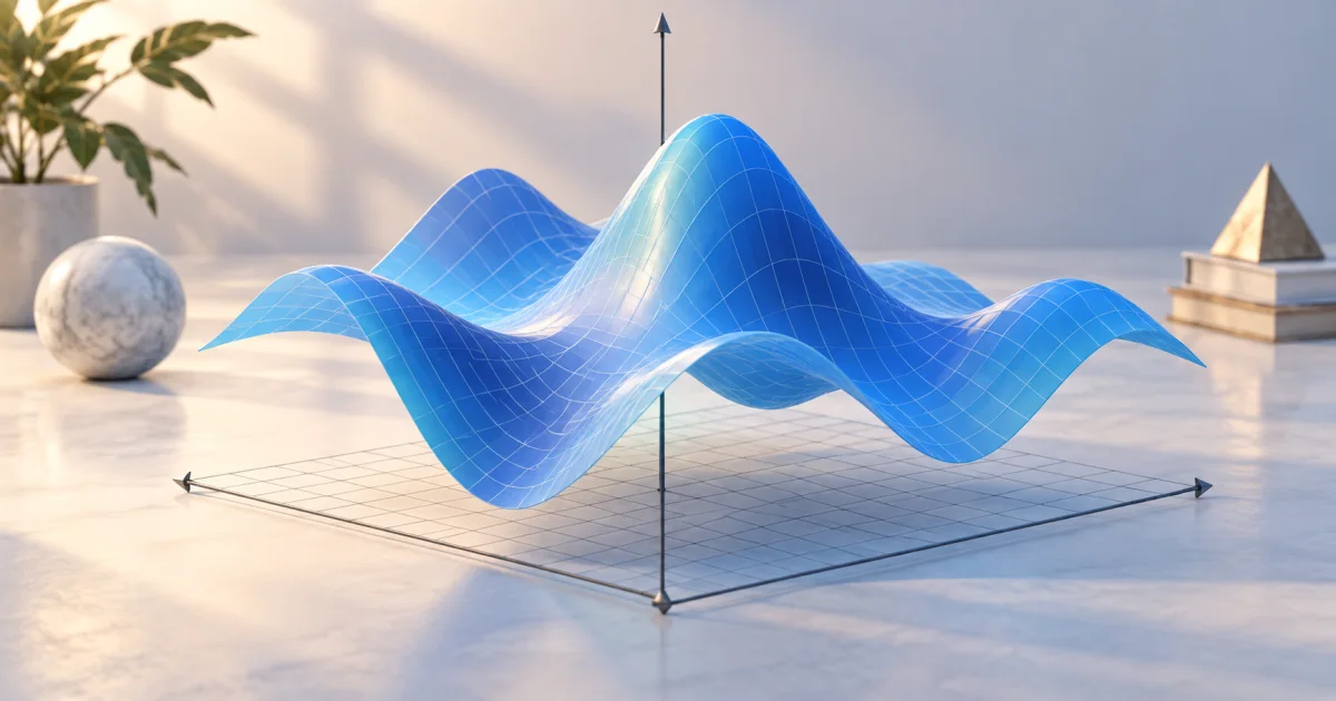
The expression exp(-(x^2 + y^2)) extends the familiar bell curve into three dimensions. It peaks at 1 at the origin and decays exponentially in all directions. The 2D Gaussian is the foundation of normal distributions in statistics, Gaussian blur in image processing, and radial basis functions in machine learning.
Practical Scenarios
Scenario 1: Calculus Student Verifying Critical Points
You solved a homework problem and found that f(x, y) = x^3 - 3xy + y^3 has critical points at (0, 0) and (1, 1). Plot x^3 - 3*x*y + y^3 in the 3D Function Plotter and rotate the surface. You can visually confirm that (0, 0) is a saddle point and (1, 1) is a local minimum -- a check that takes 5 seconds instead of computing the Hessian matrix by hand.
Scenario 2: Physics Student Visualizing Potential Fields
An electrostatic potential given by 1/sqrt(x^2 + y^2 + 0.1) models a point charge at the origin. Plotting this surface shows the steep potential well near the center and the gradual decay at large distances. Adding a second charge with 1/sqrt(x^2 + y^2 + 0.1) - 1/sqrt((x-2)^2 + y^2 + 0.1) creates a dipole field visible as two opposing peaks -- a visualization that would take 30 minutes in MATLAB.
Scenario 3: Data Scientist Exploring Loss Landscapes
Machine learning loss functions like (x^2 + y^2) + 0.5*sin(5*x)*cos(5*y) have rugged surfaces with many local minima. Plotting these surfaces reveals why gradient descent can get stuck and why techniques like momentum or learning rate scheduling matter. Change the 5 coefficient to 10 to see how increasing frequency creates a more challenging optimization landscape.
Scenario 4: Teacher Preparing Lecture Materials
Enable auto-rotate and increase resolution to 80 for a visually impressive surface. Plot 3*(1-x)^2*exp(-(x^2)-(y+1)^2) - 10*(x/5-x^3-y^5)*exp(-x^2-y^2) - 1/3*exp(-(x+1)^2-y^2) (the Peaks preset) to demonstrate a surface with multiple local maxima, minima, and saddle points in a single function. Toggle wireframe on and off to show students how surfaces are approximated by triangular meshes.
Common Mistakes and Troubleshooting
Mistake 1: Forgetting Multiplication Operators
While the parser supports implicit multiplication for patterns like 2x and 2sin(x), certain combinations require an explicit *. For example, write x*y rather than xy, because the parser reads xy as a single unknown identifier. The fix is simple: add the * operator between variables.
Mistake 2: Using Unsupported Syntax
The parser does not support |x| for absolute value -- use abs(x) instead. Similarly, ln(x) is not recognized; use log(x) for the natural logarithm. Square brackets [ and ] are not valid; use only parentheses ( and ).
Mistake 3: Ignoring Domain Restrictions
Plotting log(x) across the default range -3 to 3 produces NaN values for x <= 0, resulting in a surface with large gaps. The fix: adjust the X range to start at 0.01 or higher. Similarly, sqrt(x^2 + y^2 - 4) only produces real values where x^2 + y^2 >= 4, so expect a ring-shaped surface with a hole in the center.
Mistake 4: Setting Resolution Too High on Mobile
A resolution of 100 evaluates 10,000 grid points and generates 19,602 triangles. On older mobile devices, this can cause lag. Start at resolution 40-50 on phones and tablets. Desktop browsers handle resolution 100 smoothly.
Mistake 5: Expecting Infinite Precision Near Singularities
Functions like 1/x or tan(x) have singularities where values approach infinity. The plotter automatically converts infinity and NaN to gaps in the surface mesh. If you see missing patches, it means the function is undefined at those points -- not a bug.
Tips for Getting the Best 3D Surface Plots
- Start with a preset -- Select a preset close to your target function, then modify the expression incrementally to understand each change.
- Use the Sinc function as a test -- It is the default expression and stress-tests the plotter with a singularity at the origin and oscillations at distance.
- Widen the domain for periodic functions -- Functions involving sin and cos repeat, so expand the range to -6 or -10 to see the full pattern.
- Narrow the domain for steep functions -- Exponentials and reciprocals grow or decay fast. Use -1 to 1 or even -0.5 to 0.5 to see detail near the origin.
- Toggle wireframe to debug -- If a surface looks wrong, wireframe mode reveals whether the mesh is too coarse (increase resolution) or the function has unexpected NaN regions.
Related FindUtils Tools for Math and 3D Visualization
FindUtils offers a suite of math and visualization tools that complement the 3D Function Plotter:
- 3D Geometry Visualizer -- Explore geometric primitives (cubes, spheres, cylinders, cones) in an interactive 3D viewport. Great for spatial reasoning and geometry courses.
- 3D Vector Visualizer -- Plot vectors in 3D space, compute cross products and dot products, and visualize vector fields. Essential for multivariable calculus and physics.
- Scientific Calculator -- Evaluate complex mathematical expressions with trigonometric, logarithmic, and statistical functions. Use it alongside the plotter to compute specific function values.
- Unit Converter -- Convert between units across 20+ categories including length, area, volume, and angles. Useful when your function inputs use different unit systems.
FAQ
Q1: Is the 3D Function Plotter free to use? A: Yes. FindUtils 3D Function Plotter is available without signup, no usage limits. Processing happens entirely in your browser using WebGL -- nothing is uploaded to servers.
Q2: Is it safe to enter math expressions into an online plotter?
A: At findutils.com, the math parser uses a safe recursive descent approach -- no JavaScript eval() or Function() constructor is ever called. Only recognized mathematical tokens are processed. Your expression never leaves your device, The calculation runs locally; use synthetic data when testing sensitive workflows.
Q3: Can I plot parametric surfaces or implicit equations? A: The FindUtils plotter currently supports explicit functions in the form z = f(x, y). Parametric surfaces (where x, y, and z are each functions of parameters u and v) and implicit equations (where F(x, y, z) = 0) are not yet supported. For those, try Desmos 3D or GeoGebra 3D.
Q4: Why does my surface have holes or missing patches?
A: Holes appear where the function returns NaN (not a number) or infinity. Common causes include division by zero (e.g., 1/x at x=0), logarithm of zero or negative numbers (log(x) at x <= 0), and square roots of negative numbers. Adjust your domain to avoid these regions or accept the gaps as mathematically correct behavior.
Q5: What resolution should I use for smooth surfaces? A: A resolution of 50 (the default) works well for most functions. For presentation-quality plots, increase to 80-100. On mobile devices, stick to 40-50 to maintain smooth frame rates. Resolution 100 evaluates 10,000 points and generates nearly 20,000 triangles.
Q6: Do I need to install anything to use this tool? A: No installation is needed. The FindUtils 3D Function Plotter runs entirely in your web browser using WebGL. Any modern browser (Chrome, Firefox, Safari, Edge) on desktop or mobile works. Just open the tool and start plotting.
Next Steps
Now that you know how to plot 3D surfaces, explore more math and visualization tools on FindUtils:
- Visualize geometric solids alongside your surface plots with the 3D Geometry Visualizer
- Plot and compute vector operations in 3D space with the 3D Vector Visualizer
- Evaluate specific function values with the Scientific Calculator
- Explore other free calculators and tools in the FindUtils Calculators collection